“NaN threshold” in conservative regridding

Some datasets will contain null values (i.e. np.nan). These can propagate quite far into the computations.

To deal with this, you can use the nan_threshold keyword argument.

A demo of this is shown below, based on the Multi-Scale Ultra High Resolution (MUR) Sea Surface Temperature (SST) dataset.

Do note that if you are certain that there are no NaN values in your data, you can set skipna=False to improve performance!

For optimal memory management we want to make use of Dask’s distributed client:

from dask import distributed

c = distributed.Client()

The original dataset is of a very high resolution. We will focus on a smaller slice of the globe, and display the original data for reference:

import xarray as xr
import xarray_regrid

sst = xr.open_zarr("https://mur-sst.s3.us-west-2.amazonaws.com/zarr-v1")["analysed_sst"]

# Reduce size of array by only selecting a slice
sst = sst.sel(lat=slice(30, 45), lon=slice(125, 150)).isel(time=0)

sst.plot()

<matplotlib.collections.QuadMesh at 0x7f1dcfb66bc0>

To regrid we define a new target grid, with a lower resolution, and apply the conservative regridding with three different values for the nan_threshold:

grid = xarray_regrid.Grid(
    north=45,
    south=30,
    west=125,
    east=150,
    resolution_lat=1,
    resolution_lon=1,
)
target = grid.create_regridding_dataset(lat_name="lat", lon_name="lon")

ds0p0 = sst.regrid.conservative(target, nan_threshold=0)
ds0p5 = sst.regrid.conservative(target, nan_threshold=0.5)
ds1p0 = sst.regrid.conservative(target, nan_threshold=1)

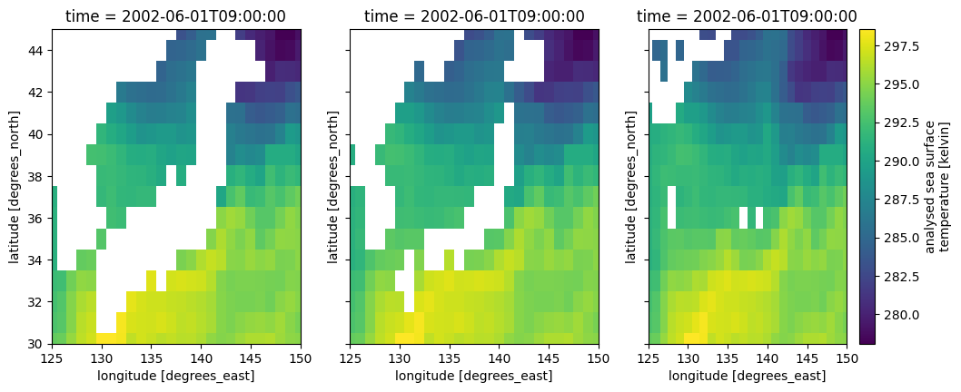
Now we can plot the data to show how the different values for nan_threshold affect the result of regridding. Note that computation will only occur in this step.

import matplotlib.pyplot as plt

fig, (ax0, ax1, ax2) = plt.subplots(ncols=3, sharex=True, sharey=True, figsize=(12, 4.5))
ds0p0.plot(ax=ax0, add_colorbar=False)
ds0p5.plot(ax=ax1, add_colorbar=False)
ds1p0.plot(ax=ax2)

ax0.set_xlim([125, 150])
ax0.set_ylim([30, 45])

(30.0, 45.0)